Chapter 1: Introduction to Random Number Generation

Random numbers play a crucial role in numerous fields including statistics, data science, machine learning, and more. However, grasping the concept of randomness can be somewhat perplexing, primarily due to its inherent unpredictability.

It's important to clarify a common misconception: the random numbers produced by computers are not genuinely random; they are termed "pseudo-random." This designation arises because these numbers are generated from long sequences of digits that are transformed into integers within a specified range. These sequences are predetermined and manipulated in various ways to simulate the experience of selecting a random number. Advanced software like MATLAB can enhance this process by factoring in elements such as the CPU or RAM time-stamp to produce a unique digit sequence. Therefore, hitting Enter should ideally yield a different “random number” each time, contingent upon the changing timestamp. However, given that there is a limited number of unique sequences that a computer can store, it is possible to eventually reproduce the same random number.

At the foundation of random number generation lies the concept of "uniform distribution." This probability distribution allows for the selection of numbers between 0 and 1, with infinite potential values existing within this range. Essentially, while there are countless numbers to choose from, they remain confined between 0 and 1 (inclusive). This distribution serves as the basis for generating random numbers across various other probability distributions.

To illustrate this, let’s say we want to generate a random number from a uniform distribution within a specific interval [a, b]. If we let X ~ U(0,1) (where X is a random number from a uniform distribution between 0 and 1), we can extend this to the interval [a, b] using the formula:

Y = a + (b-a)*X.

Here, Y will always fall within the interval [a, b]. While this method is effective, we can also explore other probability distributions.

Section 1.1: The Inverse Sampling Theorem

The inverse sampling theorem posits that for a given probability distribution p(x), if a precise inverse function exists for the probability P(X ≤ x), we can replace the value x with a uniform random number, x ~ U(0,1), and the resulting inverse function will yield a value belonging to p(x). This concept can seem intricate, so let's break it down with an example.

Consider the exponential distribution:

where λ is the inverse of the mean value (e.g., the expected value of an exponentially distributed variable X is E[X] = 1/λ). The distribution is defined as zero for x < 0, ensuring that X remains positive.

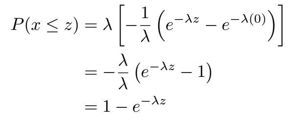
Now, if we wish to calculate the probability that X is less than or equal to a certain value z, we express this probability as follows:

Next, we modify the integral limits accordingly: the lower limit shifts from negative infinity to zero, and the upper limit changes from infinity to z, as we only want to compute the probability that X is less than or equal to z. To solve the integral, we can factor λ out as it is constant:

Using the standard integral formula, we arrive at:

This leads us to:

We can denote this function as F(z):

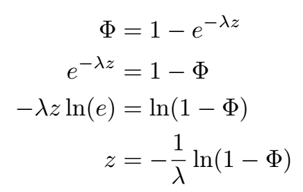
To find the inverse of this function, we want to solve for z in terms of λ, applying logarithmic rules:

or similarly:

The goal is to make z a uniformly distributed random number within [0, 1], which in turn will yield an exponentially distributed number X with a mean value of E[X] = 1/λ. Thus:

Section 1.2: Practical Application in Python

To demonstrate this concept, let's generate a sample in Python with the following code:

# Exponential random numbers

# Author: Oscar A. Nieves

# Last updated: July 01, 2021

import matplotlib.pyplot as plt

import numpy as np

plt.close('all')

np.random.seed(0) # Set seed

# Inputs

lambda1 = 0.5

samples = 10000

# Random samples (Uniformly distributed)

Z = np.random.rand(samples, 1)

# Exponential random numbers

X = -1/lambda1 * np.log(1 - Z)

# Compute mean value

EX = np.mean(X)

EX_ref = 1/lambda1

error_EX = abs(EX_ref - EX) / EX_ref

print(EX)

print(error_EX * 100)

# Plot histograms

bins = 50

plt.subplot(1, 2, 1)

plt.hist(Z, bins)

plt.xlabel('Z ~ Uniform')

plt.ylabel('Frequency')

plt.subplot(1, 2, 2)

plt.hist(X, bins)

plt.xlabel('X ~ Exponential')

plt.ylabel('Frequency')

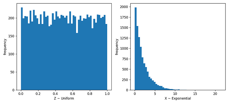
This code generates the following output:

From the results, we see that Z is uniformly distributed between 0 and 1, while X follows an exponential distribution, with a higher concentration of values nearer to 0. In this example, with λ = 0.5, the expected mean of X is E[X] = 2. The actual computed mean is approximately 1.981, resulting in a small error margin of around 0.93%. As the sample size increases beyond 10,000, this error tends to diminish, ultimately converging to the precise expected value as the number of samples approaches infinity.

This technique can be adapted to other probability distributions, provided that we can accurately compute the inverse functions for their cumulative probabilities.

Chapter 2: Practical Python Tutorials on Random Numbers

Explore practical applications of random number generation in Python through the following video tutorials.

The first video tutorial dives into generating random numbers and data using the random module in Python, providing a hands-on approach to understanding these concepts.

The second video offers quick tips on generating random numbers in Python, perfect for beginners looking to enhance their programming skills.